Note
Go to the end to download the full example code.
Iris Dataset Clustering Example#
This example is meant to illustrate the use of the Radius clustering library on the Iris dataset. It comes with a simple example of how to use the library to cluster the Iris dataset and a comparison with kmeans clustering algorithms.
The example includes: 1. Loading the Iris dataset 2. Applying Radius clustering and k-means clustering 3. Visualizing the clustering results
This example serves as a simple introduction to using the Radius clustering library on a well-known dataset.
# Author: Haenn Quentin
# SPDX-License-Identifier: MIT
Load the Iris dataset#
We start by loading the Iris dataset using the fetch_openml function from sklearn.datasets. The Iris dataset is a well-known dataset that contains 150 samples of iris flowers. Each sample has 4 features: sepal length, sepal width, petal length, and petal width. The dataset is labeled with 3 classes: setosa, versicolor, and virginica.
import numpy as np
from sklearn import datasets
from radius_clustering import RadiusClustering

# Load the Iris dataset
iris = datasets.load_iris()
X = iris["data"]
y = iris.target
Visualize the Iris dataset#
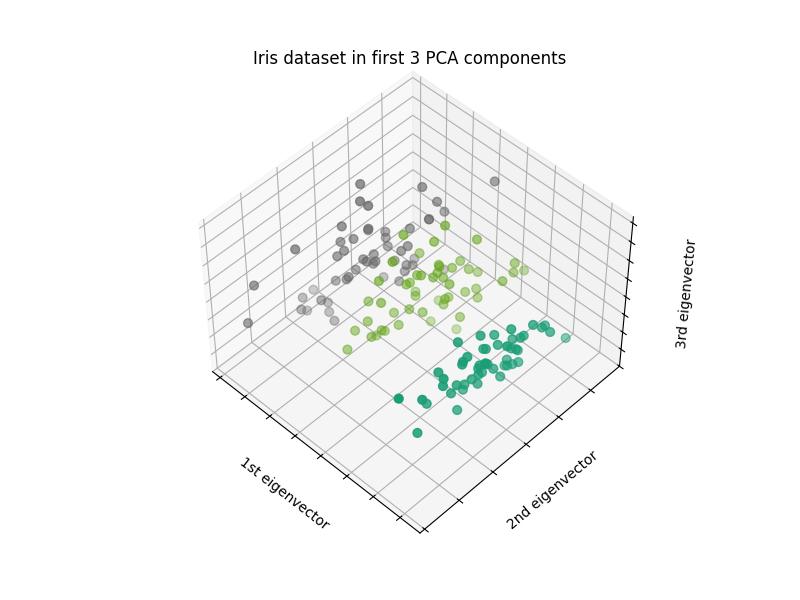
We can visualize the Iris dataset by plotting the dataset. We use PCA to reduce the dimensionality to 3D and plot the dataset in a 3D scatter plot.
import matplotlib.pyplot as plt
from sklearn.decomposition import PCA
import mpl_toolkits.mplot3d

# Reduce the dimensionality of the dataset to 3D using PCA
pca = PCA(n_components=3)
iris_reduced = pca.fit_transform(X)
fig = plt.figure(figsize=(8, 6))
ax = fig.add_subplot(111, projection="3d", elev=48, azim=134)
ax.scatter(
    iris_reduced[:, 0],
    iris_reduced[:, 1],
    iris_reduced[:, 2],
    c=y,
    cmap="Dark2",
    s=40,
)
# Set plot labels
ax.set_title("Iris dataset in first 3 PCA components")
ax.set_xlabel("1st eigenvector")
ax.set_ylabel("2nd eigenvector")
ax.set_zlabel("3rd eigenvector")

# Hide tick labels
ax.xaxis.set_ticklabels([])
ax.yaxis.set_ticklabels([])
ax.zaxis.set_ticklabels([])

plt.show()

Compute Clustering with Radius Clustering#
We can now apply Radius clustering to the Iris dataset. We create an instance of the RadiusClustering class and fit it to the Iris dataset.
import time

rad = RadiusClustering(manner="exact", threshold=1.43)
t0 = time.time()
rad.fit(X)
t_rad = time.time() - t0
Compute KMeans Clustering for Comparison#
We can also apply KMeans clustering to the Iris dataset for comparison.
from sklearn.cluster import KMeans

k_means = KMeans(n_clusters=3, n_init=10)
t0 = time.time()
k_means.fit(X)
t_kmeans = time.time() - t0
We want to have the same color for the same cluster in both plots. We can achieve this by matching the cluster labels of the Radius clustering and the KMeans clustering. First we define a function to retrieve the cluster centers from the Radius clustering and KMeans clustering and match them pairwise.
def get_order_labels(kmeans, rad, data):
    centers1_cpy = kmeans.cluster_centers_.copy()
    centers2_cpy = data[rad.centers_].copy()
    order = []
    # For each center in the first clustering, find the closest center in the second clustering
    for center in centers1_cpy:
        match = pairwise_distances_argmin([center], centers2_cpy)
        # if there is only one center left, assign it to the last cluster label not yet assigned
        if len(centers2_cpy) == 1:
            for i in range(len(centers1_cpy)):
                if i not in order:
                    order.append(i)
                    break
            break
        # get coordinates of the center in the second clustering
        coordinates = centers2_cpy[match]
        # find the closest point in the data to the center to get the cluster label
        closest_point = pairwise_distances_argmin(coordinates, data)
        match_label = rad.labels_[closest_point]
        # remove the center from the second clustering
        centers2_cpy = np.delete(centers2_cpy, match, axis=0)
        # add the cluster label to the order
        order.append(int(match_label[0]))
    return order


from sklearn.metrics.pairwise import pairwise_distances_argmin

rad_centers_index = np.array(rad.centers_)
order = get_order_labels(k_means, rad, X)

kmeans_centers = k_means.cluster_centers_
rad_centers = rad_centers_index[order]
rad_centers_coordinates = X[rad_centers]

# Pair the cluster labels
kmeans_labels = pairwise_distances_argmin(X, kmeans_centers)
rad_labels = pairwise_distances_argmin(X, rad_centers_coordinates)
Plotting the results and the difference#
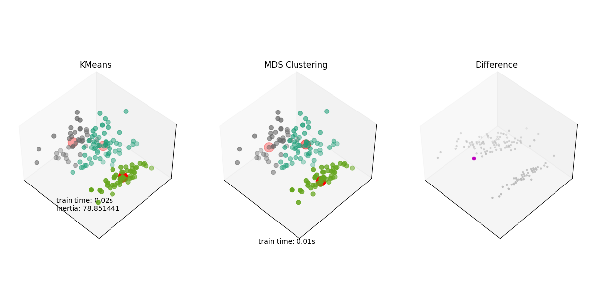
fig = plt.figure(figsize=(12, 6))
fig.subplots_adjust(left=0.02, right=0.98, bottom=0.05, top=0.9)
colors = ["#4EACC5", "#FF9C34", "#4E9A06"]

# KMeans
ax = fig.add_subplot(1, 3, 1, projection="3d", elev=48, azim=134, roll=0)

ax.scatter(
    iris_reduced[:, 0],
    iris_reduced[:, 1],
    iris_reduced[:, 2],
    c=kmeans_labels,
    cmap="Dark2",
    s=40,
)
# adapting center coordinates to the 3D plot
kmeans_centers = pca.transform(kmeans_centers)
ax.scatter(
    kmeans_centers[:, 0],
    kmeans_centers[:, 1],
    kmeans_centers[:, 2],
    c="r",
    s=200,
)
ax.set_title("KMeans")
ax.set_xticks(())
ax.set_yticks(())
ax.set_zticks(())

ax.text3D(-3.5, 3, 1.0, "train time: %.2fs\ninertia: %f" % (t_kmeans, k_means.inertia_))

# MDS
ax = fig.add_subplot(1, 3, 2, projection="3d", elev=48, azim=134, roll=0)
ax.scatter(
    iris_reduced[:, 0],
    iris_reduced[:, 1],
    iris_reduced[:, 2],
    c=rad_labels,
    cmap="Dark2",
    s=40,
)
# adapting center coordinates to the 3D plot
rad_centers_coordinates = pca.transform(rad_centers_coordinates)
ax.scatter(
    rad_centers_coordinates[:, 0],
    rad_centers_coordinates[:, 1],
    rad_centers_coordinates[:, 2],
    c="r",
    s=200,
)
ax.set_title("MDS Clustering")
ax.set_xticks(())
ax.set_yticks(())
ax.set_zticks(())
ax.text3D(-3.5, 3, 0.0, "train time: %.2fs" % t_rad)

# Initialize the different array to all False
different = rad_labels == 4
ax = fig.add_subplot(1, 3, 3, projection="3d", elev=48, azim=134, roll=0)

for k in range(3):
    different += (kmeans_labels == k) != (rad_labels == k)

identical = np.logical_not(different)
ax.scatter(
    iris_reduced[identical, 0], iris_reduced[identical, 1], color="#bbbbbb", marker="."
)
ax.scatter(iris_reduced[different, 0], iris_reduced[different, 1], color="m")
ax.set_title("Difference")
ax.set_xticks(())
ax.set_yticks(())
ax.set_zticks(())

plt.show()

Another difference plot#
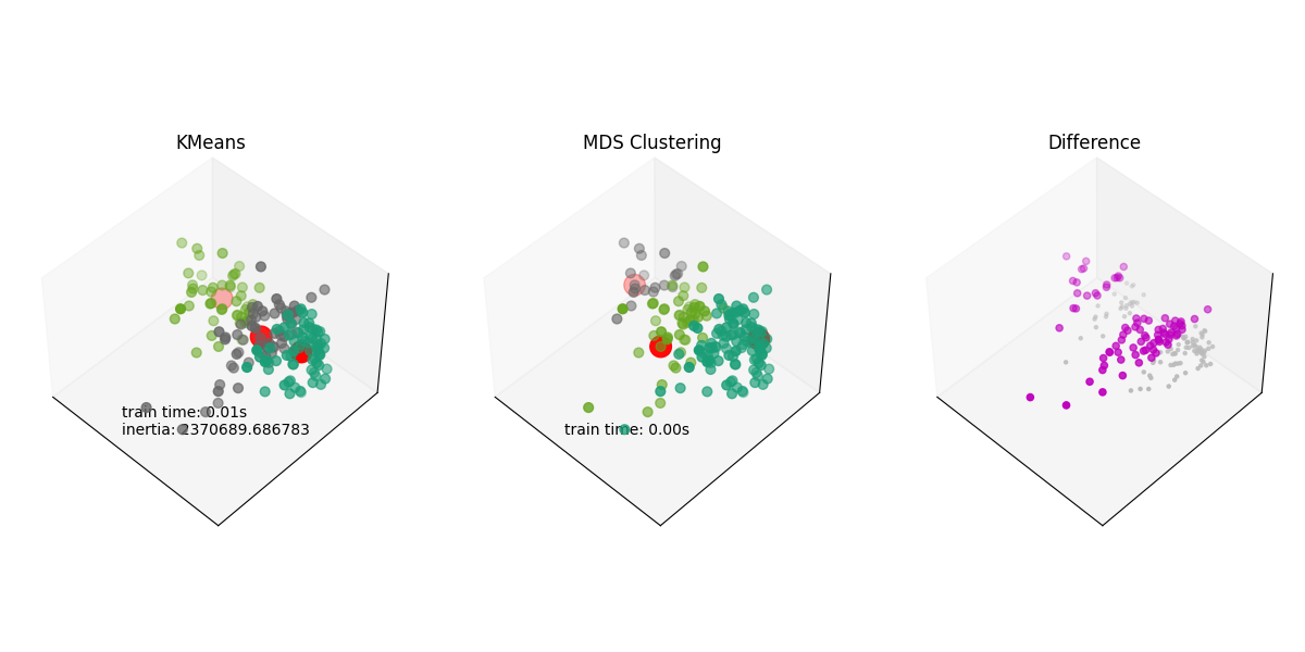
As we saw, the difference plot is not very informative using Iris. We’ll use a different dataset to show the difference plot.
wine = datasets.load_wine()
X = wine.data
y = wine.target
pca = PCA(n_components=3)
wine_reduced = pca.fit_transform(X)

# Compute clustering with MDS

rad = RadiusClustering(manner="exact", threshold=232.09)
t0 = time.time()
rad.fit(X)
t_rad = time.time() - t0

# Compute KMeans clustering for comparison

k_means = KMeans(n_clusters=3, n_init=10)
t0 = time.time()
k_means.fit(X)
t_kmeans = time.time() - t0
Reapllying the same process as before#
rad_centers_index = np.array(rad.centers_)
order = get_order_labels(k_means, rad, X)

kmeans_centers = k_means.cluster_centers_
rad_centers = rad_centers_index[order]
rad_centers_coordinates = X[rad_centers]

# Pair the cluster labels
kmeans_labels = pairwise_distances_argmin(X, kmeans_centers)
rad_labels = pairwise_distances_argmin(X, rad_centers_coordinates)
Plotting the results and the difference#
fig = plt.figure(figsize=(12, 6))
fig.subplots_adjust(left=0.02, right=0.98, bottom=0.05, top=0.9)
colors = ["#4EACC5", "#FF9C34", "#4E9A06"]

# KMeans
ax = fig.add_subplot(1, 3, 1, projection="3d", elev=48, azim=134, roll=0)

ax.scatter(
    wine_reduced[:, 0],
    wine_reduced[:, 1],
    wine_reduced[:, 2],
    c=kmeans_labels,
    cmap="Dark2",
    s=40,
)
# adapting center coordinates to the 3D plot
kmeans_centers = pca.transform(kmeans_centers)
ax.scatter(
    kmeans_centers[:, 0],
    kmeans_centers[:, 1],
    kmeans_centers[:, 2],
    c="r",
    s=200,
)
ax.set_title("KMeans")
ax.set_xticks(())
ax.set_yticks(())
ax.set_zticks(())

ax.text3D(
    60.0, 80.0, 0.0, "train time: %.2fs\ninertia: %f" % (t_kmeans, k_means.inertia_)
)

# MDS
ax = fig.add_subplot(1, 3, 2, projection="3d", elev=48, azim=134, roll=0)
ax.scatter(
    wine_reduced[:, 0],
    wine_reduced[:, 1],
    wine_reduced[:, 2],
    c=rad_labels,
    cmap="Dark2",
    s=40,
)
# adapting center coordinates to the 3D plot
rad_centers_coordinates = pca.transform(rad_centers_coordinates)
ax.scatter(
    rad_centers_coordinates[:, 0],
    rad_centers_coordinates[:, 1],
    rad_centers_coordinates[:, 2],
    c="r",
    s=200,
)
ax.set_title("MDS Clustering")
ax.set_xticks(())
ax.set_yticks(())
ax.set_zticks(())
ax.text3D(60.0, 80.0, 0.0, "train time: %.2fs" % t_rad)

# Initialize the different array to all False
different = rad_labels == 4
ax = fig.add_subplot(1, 3, 3, projection="3d", elev=48, azim=134, roll=0)

for k in range(3):
    different += (kmeans_labels == k) != (rad_labels == k)

identical = np.logical_not(different)
ax.scatter(
    wine_reduced[identical, 0], wine_reduced[identical, 1], color="#bbbbbb", marker="."
)
ax.scatter(wine_reduced[different, 0], wine_reduced[different, 1], color="m")
ax.set_title("Difference")
ax.set_xticks(())
ax.set_yticks(())
ax.set_zticks(())

plt.show()

Conclusion#
In this example, we applied Radius clustering to the Iris and Wine datasets and compared it with KMeans clustering. We visualized the clustering results and the difference between the two clustering algorithms. We saw that Radius Clustering can lead to smaller clusters than kmeans, which produces much more equilibrate clusters. The difference plot can be very useful to see where the two clustering algorithms differ.
Total running time of the script: (0 minutes 0.458 seconds)
Related examples
